Figures and Charts

Figure 1: Pix4D help menu


Figure 3: Acquisition Pattern of Truck Model

Figure 4: NADIR view of 3D Model

Figure 5: Right side view of 3D Model

Figure 6: Left side view of 3D Model

Figure 7: Sundarbans Mangrove Region

Figure 8: Shows Color Infrared Band Combination
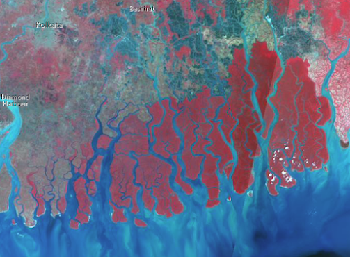
Figure 9: Color Infrared Of Mangrove Forest

Figure 10: Takla Makan Desert

Figure 11: Takla Makan Desert With Moisture Index

Figure 12: Shows Moisture Index


Figure 14: Las Vegas In 2021

Figure 15: Shows Pix4D New Mission Page

Figure 16: Shed Where Operation Was Conducted

Figure 17: Uploading Images To Pix4D Mapper

Figure 18: Image Properties Page


Figure 20: Selecting The Type Of Project

Figure 21: NADIR Top-Down View

Figure 22: NADIR Front View

Figure 23: NADIR Side View

Figure 24: NADIR Back View

Figure 25: 60° Top-Down View

Figure 26: 60° Front View
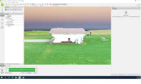
Figure 27: 60° Side View

Figure 28: 60° Back View

Figure 29: Propeller Aeropoints

 Figure 31: Uploading Data To Software


Figure 30: Sketch Of Operation Area
Figure 32: Image Properties Page
Figure 33: Selecting Output Coordinate System

Figure 34: Selecting The Type Of Project


Figure 36: West Facing View

Figure 37: Surrounding Area Of Mock Accident

Figure 38: Top-Down View Of Mock Accident

Figure 39: Micasense RedEdge Peak Band Reflectance

Figure 40: Color Ramp Related to Pixel Reflection

Figure 41: Shows PWA With False Color IR Pre-Burn

Figure 42: Shows The Swipe Tool In Use

Figure 43: Shows The Swipe Tool In Use

Figure 44: Shows Post-Burn-NDVI With Inverted Color Scheme

Figure 45: Shows The Regular Post-Burn And NDVI Post-Burn

Figure 46: Shows Zoomed In Plot That Didn't Fully Burn

Figure 47: Shows The Color Band Combination I Generated

Figure 48: Shows The GCP Data File We Will Be Working With

Figure 49: Shows XY Point Data On The Add Data Icon

Figure 50: Shows First XY Parameters

Figure 51: Shows The Correct Parameter Settings

Figure 52: Shows GCP Points On The Basemap

Figure 53: Shows The Points And Terrain Features

Figure 54: Shows The Points And Terrain Features

Figure 55: The Search Bar

Figure 56: Longitude And Latitude Lines

Figure 57: Demonstrate Projection

Figure 58: Flight Area At Purdue Wildlife Area

Figure 59: Shows Location Of Ground Control Points

Figure 60: Shows Image Properties Page

Figure 61: Data Loaded In And Beginning Initial Processing

Figure 62: Shows Uncalibrated Images

Figure 63: GCP/MTP Manager Window

Figure 64: Shows Manual GCP Correction

Figure 65: The Map With GCPs After It Was Reoptimized

Figure 66: The Final Product After initial processing, GCPs added, reoptimized, point cloud/mesh, and DSM, orthomosaic, and index have finished

Figure 67: Orthomosaic Imagery Of PWA
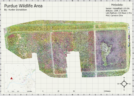
Figure 68: Purdue Wildlife Area Map

Figure 69: Wolf Paving Excavation Map

Figure 70: Map example from Esri tutorial

Figure 71: Measure Area Tool

Figure 72: Select Layer By Location Results

Figure 73: Composite Bands Tool

Figure 74: False IR of PWA

Figure 75: Final Product

Figure 76: Example of Attribute Table

Figure 77: Health Care Facilities In Washington

Figure 78: Health Care Facilities Attribute Table
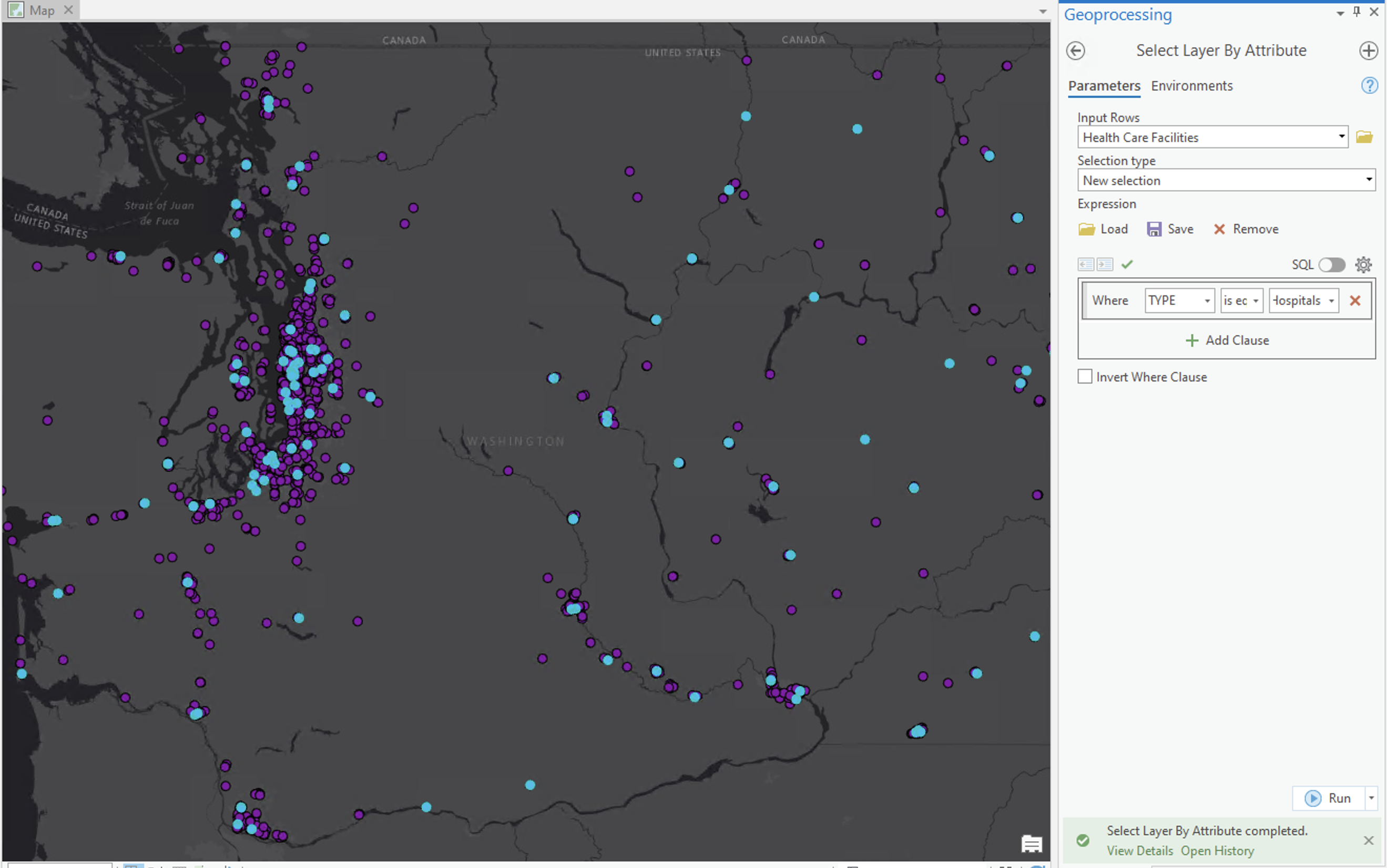
Figure 79: All Hospitals Identified

Figure 80: Hospitals With 200 Or More Cases Of Influenza

Figure 81: Proposed Wilderness Study Area

Figure 82: Selected Wilderness Areas

Figure 83: Field Acres Statistics

Figure 84: Four Different Features

Figure 85: PILOT_CERT Standalone Table

Figure 86: Airman Points By Different Types

Figure 87: All Pilots In The United States

Figure 88: All Commercial Pilots In The United States

Figure 89: Airmen In Indiana

Figure 90: All Pilots In Indiana By Counties

Figure 91: Stateboundaries In Lambert

Figure 92: Kernel Density For Airman In Indiana

Figure 93: Indiana Counties Clipped

Figure 94: Fishnet_10km Clipped

Figure 95: Indiana Airmen Spatial Analysis

Figure 96: Continental United States Analysis

Figure 97: Slope Visual

Figure 98: Aspect Visual

Figure 99: Slope Raster Over San Diego

Figure 100: Aspect Raster Over San Diego

Figure 101: Binary Suitability Analysis of San Diego.

Figure 102: Hillshading Visual

Figure 103: Hillside Elevation Surface

Figure 104: Contour Lines At Specific Elevations

Figure 105: 3D Scene Linked To 2D Scene

Figure 106: LightLocations Attribute Table

Figure 107: Viewshed 3D Analysis

Figure 108: Model Light Schemes With New Values

Figure 109: Construct Sight Lines

Figure 110: After Sight Lines Above 1,100 Removed

Figure 111:Visibility Distance Excludes Over 600ft

Figure 112: Litchfield Dredge 7/4/17

Figure 113: Litchfield Dredge 7/22/17

Figure 114: Litchfield Dredge 8/27/17

Figure 115: Wolfcreek After Extraction

Figure 116: Wolfcreek Elevation Surface Information

Figure 117: Wolfcreek Stock Pile Volumetric

Figure 118: Litchfield Volume Analysis at 2cm

Figure 119: Litchfield Volume Analysis at 10cm

Figure 120: Litchfield Volume Analysis at 100cm

Figure 121: Parameters For Extracting Bands

Figure 122: After Bands Are Extracted

Figure 123: Segmented Preview

Figure 124: Shows All Samples Collected

Figure 125: Shows The Classification Preview

Figure 126: Shows Data After The Merge

Figure 127: Final Classification Map

Figure 128: Shows Reclassify Tool For Pixel Count

Figure 129: Classification Of Tippecanoe Country Amphitheater

Figure 130: Tippecanoe Country Amphitheater Impervious and Pervious

Figure 131: Tippecanoe Country Amphitheater Road Crack

Figure 132: Add GCP Point

Figure 133: Every Crews GCP Points Marked

Figure 134: GCP Locations For Mock Operation

Figure 135: Mock Mission Area

Figure 136: Mock Operation Metadata

Figure 137: Golf Course Locator Map

Figure 138: Front of Clubhouse

Figure 139: Left Side of Clubhouse

Figure 140: Back of Clubhouse

Figure 141: Right Side of Clubhouse

Figure 142: Top of Clubhouse

Figure 143: Overview of Clubhouse

Figure 145: 3D Model Quality Report

Figure 146: Flight Operation Area

Figure 147: GCP Location Variability

Figure 148: Flight 1 Quality Report

Figure 149: Flight 2 Quality Report

Figure 150: First Data Collection at PWA

Figure 151: Second Data Collection At PWA

Figure 152: Side-By-Side Orthomosaic

Figure 153: Classification For Flight 1

Figure 154: Classification For Flight 2

Figure 155: Side-By-Side Classification
Comments
Post a Comment